
Alloy 263: When CALPHAD Results Need Engineering Judgment
A practical study of γ′/η competition, phase-model interpretation and melting-range validation
Computational thermodynamics can reveal phase stability, precipitation tendencies and melting behavior long before an experimental campaign is completed. But a converged CALPHAD calculation is not automatically a reliable engineering result. A recent KERRIUM study of Alloy 263 illustrates why.
What began as a straightforward equilibrium calculation produced two unexpected results: an apparently enormous γ′ fraction at elevated temperature and, later, an isolated prediction of 100% liquid at 1288°C. Both calculations converged. Neither could be accepted at face value.
The investigation became a useful demonstration of a central principle of digital metallurgy: the value of a calculation lies not only in producing a result, but in knowing how to interrogate, validate and interpret it.
Why Alloy 263?
Alloy 263 is a Ni-Co-Cr wrought superalloy combining high-temperature strength, oxidation resistance, weldability and fabricability. Haynes lists a nominal composition around 52Ni-20Cr-20Co-6Mo-2.4Ti-0.4Al wt.%, with smaller additions and controlled residuals [1].
Its principal strengthening precipitate is ordered L1₂ γ′, approximately represented as:
γ′ ∼ Ni3(Al,Ti)
However, its microstructural stability involves more than γ and γ′. η phase and carbides such as M₂₃C₆ can become important depending on temperature and exposure history.
This makes Alloy 263 particularly useful for testing not just a CALPHAD calculation, but the interpretation of a CALPHAD calculation.
The first calculation — and the first warning
Using pycalphad and a multicomponent Ni-alloy thermodynamic database, an equilibrium calculation was performed with γ, γ′, η, carbides, TCP phases and liquid included as candidate phases.
The first phase-fraction diagram appeared reasonable—until an intermediate temperature range showed almost the entire alloy labelled γ′. At approximately 1100°C:
fγ′ ≈ 99%
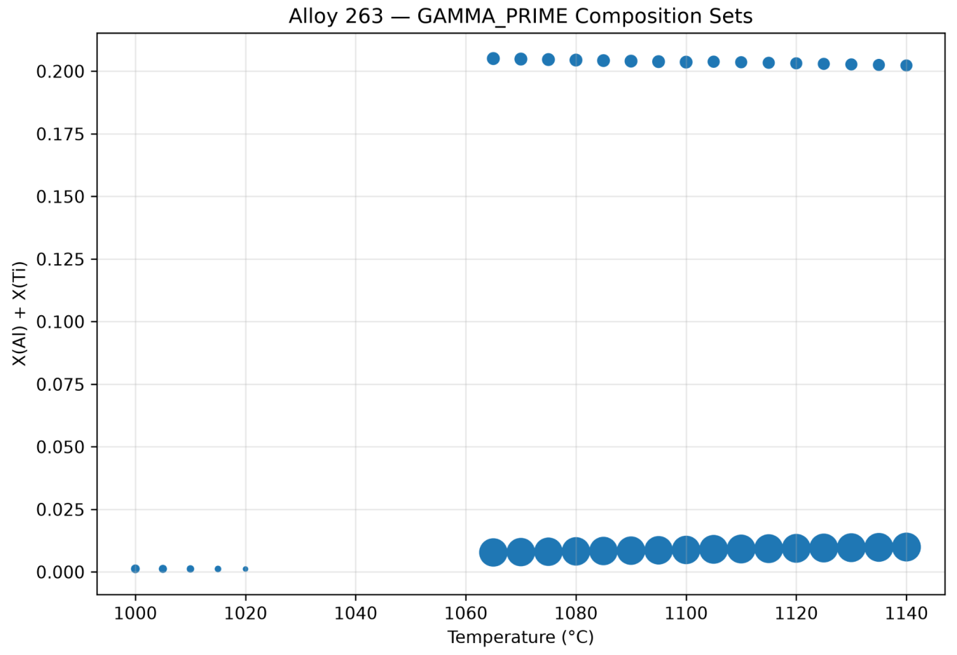
For Alloy 263, this immediately required investigation. Instead of accepting the phase label, the individual equilibrium composition sets were inspected.
Two different states carrying the same γ′ label were present. One accounted for approximately 84% of the alloy and was rich in Ni, Cr and Co with almost no Ti. The second accounted for approximately 15% and was strongly enriched in Ni, Ti and Al. The two states clearly did not represent the same metallurgical object.
Looking inside γ′
The database describes γ′ with a two-sublattice model having a 0.25:0.75 site ratio, appropriate for representing an ordered L1₂-type phase. Examining the calculated site occupancies was therefore more informative than reading the phase name alone. For the γ′-like composition set at 1100°C, the first sublattice showed strong Ti and Al occupancy:
YTi(0) ≈ 0.664, YAl(0) ≈ 0.151
while the second sublattice was overwhelmingly occupied by Ni:
YNi(1) ≈ 0.900
This is characteristic of strongly ordered Ni₃(Al,Ti)-type γ′. The much larger γ′ composition set showed a fundamentally different ordering pattern.
The lesson is important: a database phase name is not, by itself, sufficient microstructural identification. For ordered phases, composition sets and sublattice occupancies may be essential to interpreting the calculation correctly.
γ′–η competition
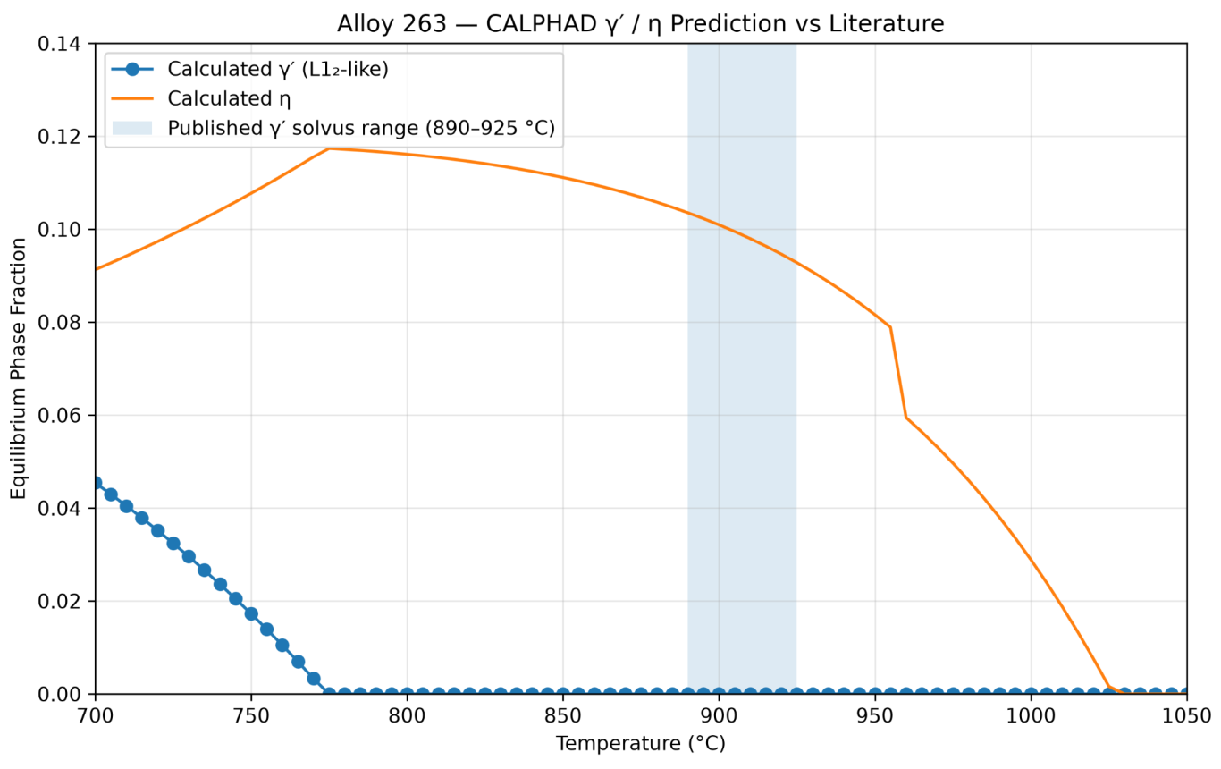
The next step was to distinguish L1₂-like γ′ states using their calculated ordering characteristics and then repeat the equilibrium calculation with η included.
This is metallurgically meaningful. Published work on Alloy 263 reports η precipitation during long-term thermal exposure, with η formation occurring at the expense of γ′ [2,4]. Long-term exposure experiments at 800°C have also demonstrated the development of η precipitates and their influence on creep behavior [4].
However, quantitative validation revealed a limitation. Published literature places the γ′ solvus of C-263 approximately within [3]:
890°C < Tγ′solvus < 925°C
In the present calculation, the identified L1₂-like γ′ was suppressed substantially earlier when η was allowed to equilibrate.
The database therefore appears to reproduce an important qualitative mechanism—γ′/η competition—while not providing sufficiently convincing quantitative γ′ stability for this particular Alloy 263 calculation.
That distinction matters. A model can capture the right physics qualitatively without yet being accurate enough for a quantitative heat-treatment recommendation.
Equilibrium is not a heat-treatment simulation
There is another reason not to equate the equilibrium diagram with the actual microstructure. Equilibrium thermodynamics asks: which state minimizes G at a given T,P, and composition? A heat-treatment problem asks something different: what can nucleate, grow, dissolve or transform within a finite time? η may be thermodynamically favored but kinetically slow to form. Indeed, published Alloy 263 work reports slower precipitation kinetics for η than for γ′. Consequently:
Equilibrium phase stability ≠ heat-treated microstructure
For heat-treatment design, thermodynamics must ultimately be connected to precipitation kinetics and time-temperature history.
A second warning: the 1288°C liquid anomaly
The melting calculation produced another useful diagnostic challenge.
The initial equilibrium output contained:
1286°C: fL = 0
1288°C: fL = 1
1290°C: fL ≈ 0.00045
A material cannot become completely liquid and then almost completely solid again as temperature increases under the same equilibrium conditions.
The 1288°C result was therefore rejected as a numerical/model-state anomaly rather than interpreted as metallurgy. For the melting region, the calculation was repeated with the physically relevant high-temperature phases restricted to:
FCC_A1 + LIQUID
and with a finer temperature increment.
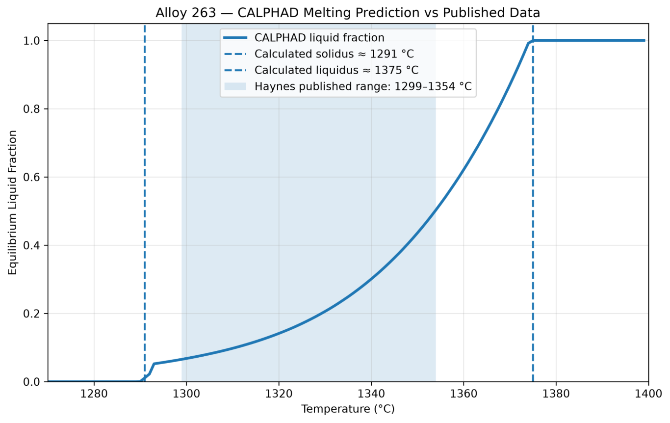
The anomaly disappeared. The liquid fraction then increased continuously with temperature.
Melting-range validation
The refined calculation produced approximately:
Tsolidus ≈ 1291°C
Tliquidus ≈ 1375°C
or an equilibrium melting interval of approximately:
84°C
Haynes publishes a melting range of 2370–2470°F for Alloy 263, approximately 1300–1355°C [1].
The comparison is instructive:
Parameter CALPHAD Published Difference
Solidus 1291°C ≈1300°C ≈−9°C
Liquidus 1375°C ≈1355°C ≈+20°C
Melting interval 84°C ≈55°C ≈+29°C
The predicted onset of melting is reasonably close to the published value. The calculated liquidus is higher, producing a wider predicted melting interval. This is a much more useful statement than simply reporting “1291–1375°C.” The calculation has been benchmarked, and its deviation is visible.
What this case teaches
Several practical conclusions emerge from this exercise.
Solver convergence is not validation. A numerically successful equilibrium calculation can still contain a physically implausible solution.
Database quality is application-dependent. An open thermodynamic database can be extremely valuable for learning, screening and mechanism exploration while still requiring caution for quantitative engineering predictions in a specific commercial superalloy.
Phase labels require interpretation. For ordered phases such as γ′, composition sets and sublattice occupancies can contain information that a conventional phase-fraction plot hides.
Equilibrium and kinetics must be separated. Thermodynamic stability establishes what is possible at equilibrium; it does not determine what will form during a practical heat treatment.
Reference data are part of the computational workflow. Validation should not be an afterthought performed after a graph has been published.
From CALPHAD to Digital Metallurgy
This case suggests a practical definition of digital metallurgy. It is not simply the use of CALPHAD software.
A useful workflow is:
Composition→Thermodynamic Prediction→Model Interrogation→Validation→Engineering Interpretation
The next layer extends the chain:
Thermodynamics→Kinetics→Microstructure→Properties→Engineering Decision
That is the direction in which a digital materials library becomes more than a collection of datasheets. It becomes a framework for connecting materials data, computational metallurgy and engineering judgment.
Conclusion
The Alloy 263 calculation did not produce a perfect answer—and that is precisely why it became useful.
An unexpected γ′ result forced examination of composition sets and sublattice ordering. γ′–η competition demonstrated the difference between capturing a mechanism and predicting it quantitatively. An isolated liquid-state anomaly demonstrated the need for numerical sanity checks. Finally, comparison with published melting data provided a measurable assessment of model accuracy.
The central lesson is simple:
Digital metallurgy is not about generating more calculations. It is about knowing which calculations to trust.
References
[1] Haynes International, Inc. HAYNES® 263 Alloy. Manufacturer technical data and alloy brochure. Nominal composition, physical properties, fabrication information and published melting range of 2370–2470°F (approximately 1300–1355°C).
[2] Zhao, J.-C., Ravikumar, V., and Beltran, A. M. “Phase Precipitation and Phase Stability in Nimonic 263.” Metallurgical and Materials Transactions A, Vol. 32, 2001, pp. 1271–1282. DOI: 10.1007/s11661-001-0217-4.
[3] “Design of a New Wrought CrCoNi-Based Medium-Entropy Superalloy C-264 for High-Temperature Applications.” Materials & Design, 2021. C-263 is used as a reference alloy, including comparison of γ′ solvus behavior.
[4] “The Effect of η Phase Precipitates on the Creep Behavior of Alloy 263 and Variants.” Materials Science and Engineering A, Vol. 799, 2021, 140337. DOI: 10.1016/j.msea.2020.140337.
Methodology note: CALPHAD results presented in this study were generated using pycalphad with an open multicomponent thermodynamic database. Calculated values are model- and database-dependent and should not be interpreted as certified material properties. Published manufacturer data and peer-reviewed experimental literature were used for validation and engineering interpretation.